Solving the Lorenz equations using an analog circuit

Introduction

Nonlinear and chaotic systems are often governed by seemingly simple rules, yet produce astonishingly rich behavior. The Lorenz system is a classic example. It originated from Edward Lorenz’s simplified model of atmospheric convection and was pioneering work in the development of chaos theory. It has always captivated me and many others.

I recall seeing an analog circuit that implemented the Lorenz system at an APS conference some years back, and I have always wanted to replicate it ever since. I finally did. I’d like to share details about the build and design for others who want to build one for themselves. Other tutorials I found online didn’t go into sufficient detail about how the circuit worked, from equations to components.

Hopefully this will help others who want to understand in depth why it works, rather than just following a given circuit diagram on faith. I hope the reader will take away from this article not just an understanding of this particular implementation, but a framework that generalizes and allows them to apply it to other differential equations of interest. If you’re interested in dynamical systems, analog computing, and electronics, this is a really fun and simple build, and it’s so satisfying to see the Lorenz attractor come to life on an oscilloscope.

I learned a lot from this book: A Concise Guide to Chaotic Electronic Circuits by Arturo Buscarino et al. I followed its methodology of systematically going from equation to circuit. The book does cover the Lorenz system and comes up with a circuit diagram. However, I decided on a simpler circuit design based on one from Paul Horowitz at Harvard University, discussed in this video and the associated article. My build differs in its choice of resistor values (scaled by a constant factor that doesn’t affect the dynamics) based on the resistors I had on hand. I also used different multiplier and op-amp components, but they are functionally the same.

The Lorenz system is governed by this set of differential equations:

$\frac{dx}{dt} = \sigma (y - x)$

$\frac{dy}{dt} = x(\rho - z) - y$

$\frac{dz}{dt} = xy - \beta z$

and the standard parameter choice which demonstrates chaos is

$\sigma = 10, \qquad \rho = 28, \qquad \beta = \frac{8}{3}.$

What makes this system especially interesting in hardware is that the equations map naturally onto analog computing blocks. Voltages represent the state variables $x(t)$, $y(t)$, and $z(t)$. Op-amp integrators and summing stages implement the linear pieces of the dynamics, while analog multipliers generate the nonlinear $xy$ and $xz$ terms. With the right scaling, the circuit continuously solves the differential equations in real time.

From dimensionless equations to voltages and seconds

The Lorenz equations above are dimensionless — $x$, $y$, $z$, and $t$ are all pure numbers. To map them onto an analog circuit we need to give the state variables units of voltage and time units of seconds. We do this with the following change of variables.

Let $X$, $Y$, $Z$ (in volts) and $\tau$ (in seconds) be the dimensionful counterparts, related to the dimensionless variables by

$X = k_1\, x, \qquad Y = k_2\, y, \qquad Z = k_3\, z, \qquad t = \kappa\, \tau.$

Here $k_1$, $k_2$, $k_3$ are voltage scale factors and $\kappa$ is a rate with units of $1/\text{s}$. Equivalently $\tau = t/\kappa$: one unit of dimensionless time corresponds to $1/\kappa$ seconds of real time.

For this build I take

$k_1 = k_2 = k_3 \equiv k = \tfrac{1}{10}\,\text{V}.$

With the standard parameters the dimensionless states stay roughly within $|x|, |y| \lesssim 30$ and $0 \lesssim z \lesssim 50$, so $|X|, |Y| \lesssim 3\,\text{V}$ and $0 \lesssim Z \lesssim 5\,\text{V}$ — comfortably inside the $\pm 12\,\text{V}$ supply rails of the op-amps and multipliers, with enough headroom to avoid clipping.

Substituting $x = X/k$, $y = Y/k$, $z = Z/k$, and $t = \kappa \tau$ into the dimensionless equations and tidying up gives the dimensionful system:

$\frac{dX}{d\tau} = \kappa\, \sigma\, (Y - X)$

$\frac{dY}{d\tau} = \kappa\, \rho\, X \;-\; \kappa\, Y \;-\; \frac{\kappa}{k}\, X Z$

$\frac{dZ}{d\tau} = \frac{\kappa}{k}\, X Y \;-\; \kappa\, \beta\, Z.$

A quick units check: every term on the right-hand side works out to volts per second, as it must for the derivative of a voltage. The linear terms carry one factor of $\kappa$ (with units $1/\text{s}$), and the bilinear terms carry $\kappa/k$ which has units of $(1/\text{s})\cdot(1/\text{V})$ — exactly what is needed for a product like $XY$ or $XZ$ (volts²) to come out in volts per second.

Two separate design choices live in these equations:

• $\kappa$ sets the speed. It will be set by the integrator time constant in the next section. Smaller $\kappa$ slows the attractor down; larger $\kappa$ speeds it up. Choosing $\kappa$ in the range of $10$–$1000\,\text{s}^{-1}$ produces an attractor that evolves on a millisecond-to-tenths-of-a-second timescale — slow enough to watch unfold on a scope, fast enough to look continuous.
• $k$ sets the amplitude. The choice $k = \tfrac{1}{10}\,\text{V}$ keeps the state voltages in the few-volt range, well within rail. It is also chosen to line up with the AD633 analog multiplier’s built-in $10\,\text{V}$ scale factor (in the denominator of its transfer function), which keeps the product-term resistors clean — as we’ll see when we wire up those terms.

The building block: a summing integrator

Every one of the three equations is built from the same circuit: an op-amp with several input resistors $R_1, \dots, R_N$ feeding its inverting input, a capacitor $C$ in the feedback path, and the non-inverting input grounded. With an ideal op-amp the inverting input sits at a virtual ground, so the current through each input resistor is simply $V_i / R_i$ — independent of all the others. Since no current flows into the op-amp itself, every bit of it has to flow through the capacitor. That single node equation is the entire device:

$\frac{dV_\text{out}}{d\tau} = -\sum_{i} \frac{1}{R_i C}\, V_i.$

To turn this relation into actual resistor values, it helps to write it a second way. Multiply both sides by $R_0 C$ for some reference resistance $R_0$. The rate we defined earlier is exactly $\kappa = 1/(R_0 C)$, so that prefactor is just $1/\kappa$:

$\frac{1}{\kappa}\, \frac{dV_\text{out}}{d\tau} = -\sum_{i} \frac{R_0}{R_i}\, V_i.$

Now the entire time scale sits in the single $1/\kappa$ on the left, and every coefficient on the right is a pure resistance ratio $R_0/R_i$. Sizing a stage becomes almost mechanical: write the equation it has to implement in this same $\tfrac{1}{\kappa}\dot V = \cdots$ form, and whatever number multiplies an input is that input’s ratio $R_0/R_i$. I’ll fix the reference at $R_0 = 100\,\text{k}\Omega$ throughout, so each resistor follows from $R_i = R_0 / (\text{its coefficient})$.

The three stages

Each Lorenz equation becomes one integrator stage. For each, I take its dimensionful equation from above, multiply through by $1/\kappa$ to expose the resistance ratios, and read off the resistors. The signs work out so that the stages output $X$, $-Y$, and $Z$ — exactly the polarities their neighbors need, with no standalone inverters.

The X stage

Multiplying $dX/d\tau = \kappa\, \sigma\, (Y - X)$ by $1/\kappa$ and putting in $\sigma = 10$:

$\frac{1}{\kappa}\frac{dX}{d\tau} = 10\,Y - 10\,X.$

The two inputs are $-Y$ and the fed-back output $X$. Both coefficients are $10$, so both want $R_0/R = 10$:

$R_1 = R_2 = \frac{R_0}{10} = \frac{100\,\text{k}\Omega}{10} = 10\,\text{k}\Omega.$

The Y stage

Multiplying $dY/d\tau = \kappa\, \rho\, X - \kappa\, Y - (\kappa/k)\, XZ$ by $1/\kappa$, with $\rho = 28$:

$\frac{1}{\kappa}\frac{dY}{d\tau} = 28\,X \;-\; Y \;-\; \frac{1}{k}\,XZ.$

The first two terms read off directly: $R_0/R_3 = 28$ gives $R_3 = 100\,\text{k}\Omega / 28 = 3.57\,\text{k}\Omega$, and $R_0/R_5 = 1$ gives $R_5 = 100\,\text{k}\Omega$. The product term needs one extra step, because the AD633 returns not $XZ$ but $XZ/(10\,\text{V})$. Rewriting against that actual input, with $k = \tfrac{1}{10}\,\text{V}$:

$\frac{1}{k}\,XZ = \frac{10\,\text{V}}{k}\cdot\frac{XZ}{10\,\text{V}} = 100\cdot\frac{XZ}{10\,\text{V}}.$

So the multiplier path carries coefficient $100$, and $R_4 = R_0/100 = 1\,\text{k}\Omega$. Choosing $k = \tfrac{1}{10}\,\text{V}$ to line up with the multiplier’s built-in $10\,\text{V}$ is what lands this path on a clean $1\,\text{k}\Omega$.

The Z stage

Multiplying $dZ/d\tau = (\kappa/k)\, XY - \kappa\, \beta\, Z$ by $1/\kappa$, with $\beta = \tfrac{8}{3}$:

$\frac{1}{\kappa}\frac{dZ}{d\tau} = \frac{1}{k}\,XY \;-\; \frac{8}{3}\,Z = 100\cdot\frac{XY}{10\,\text{V}} \;-\; \frac{8}{3}\,Z.$

The product path repeats the $Y$-stage trick, so $R_6 = R_0/100 = 1\,\text{k}\Omega$. The decay term gives $R_0/R_7 = \tfrac{8}{3}$, so

$R_7 = \frac{R_0}{8/3} = \tfrac{3}{8}\,R_0 = 37.5\,\text{k}\Omega.$

Notice the pattern: every resistor came out as $R_0$ divided by a Lorenz coefficient, so $R_i \times (\text{coefficient}) = 100\,\text{k}\Omega$ across the board. The odd-looking $3.57\,\text{k}\Omega$ and $37.5\,\text{k}\Omega$ are just $\rho$ and $\beta$ in disguise. Only the product $R_0 C$ is pinned down, through $\kappa = 1/(R_0 C)$: with $R_0 = 100\,\text{k}\Omega$ and a watchable $\kappa = 400\,\text{s}^{-1}$, the integrating capacitor is $C = 1/(\kappa R_0) = 25\,\text{nF}$.

The multipliers

Each product term comes from an AD633 analog multiplier. The AD633 computes the following in an analog fashion: $W = (X_1 - X_2)(Y_1 - Y_2)/(10\,\text{V}) + B$, where $B$ is a summing input added straight to the output — grounding it ($B = 0$) leaves a clean scaled product. Choosing which difference input carries the negative sign, one multiplier forms $-XZ/10\,\text{V}$ for the $Y$ stage and a second forms $-XY/10\,\text{V}$ for the $Z$ stage:

Putting it all together

That is the whole design — there is no separate master schematic to untangle. Each block was built to expose exactly the signals its neighbors need, so the complete circuit is just these stages and multipliers with their outputs wired to the matching inputs. The only feedback already drawn in the stage diagrams is each integrator’s capacitor; the resistive connections — including each stage’s own output looping back through its input resistor, which forms the linear decay term — still have to be wired. Each output goes to:

• $X$ → the $X$ stage, the $Y$ stage, and both multipliers
• $-Y$ → the $Y$ stage, the $X$ stage, and the $XY$ multiplier
• $Z$ → the $Z$ stage and the $XZ$ multiplier
• $-XZ/10\,\text{V}$ → the $Y$ stage
• $-XY/10\,\text{V}$ → the $Z$ stage

Because each stage outputs the sign its consumers need, no separate inverting amplifiers are required anywhere. Wire those connections together and the loop solves the Lorenz equations on its own.

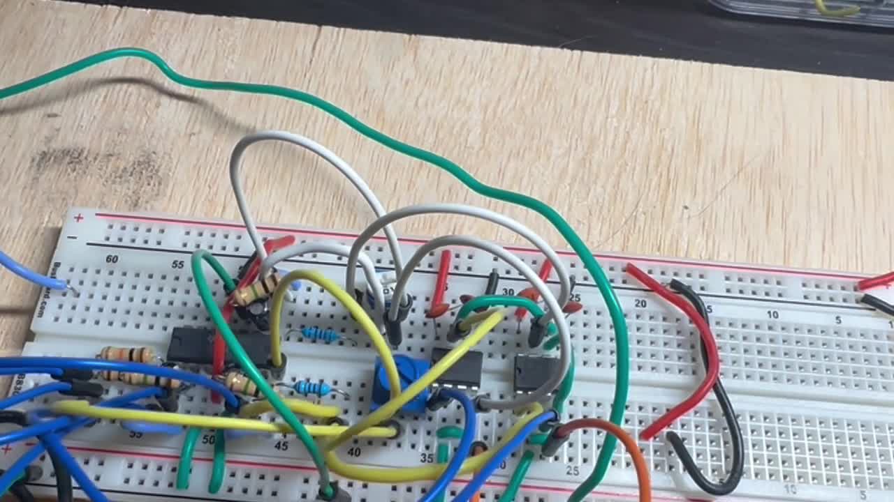
The Build

The whole thing is a short parts list. The two product terms run through a pair of AD633 analog multipliers, and the three integrators share a single TL084CN, a quad op-amp. The multipliers are the most expensive component at around $18 each; everything else is standard resistors, capacitors, and that one op-amp chip. It’s remarkable how few components it takes to continuously solve the Lorenz equations in real time.

For power, I used two 12V DC adapters wired in series: I connected the negative terminal of one adapter to the positive terminal of the other, and that junction becomes the common ground (0V). This gives the three voltage levels needed for the op-amp and multiplier rails — the free positive terminal sits at +12V and the free negative terminal at −12V relative to that ground.

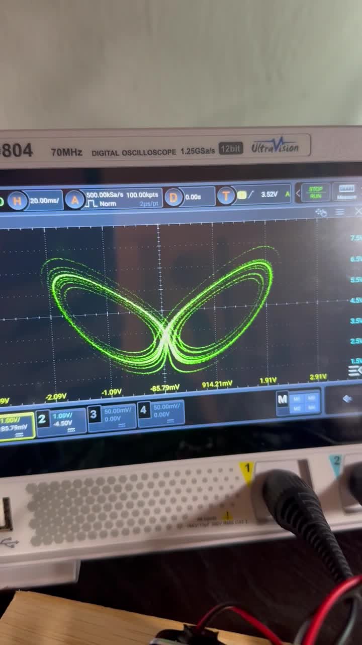
Oscilloscope Capture

Once the circuit is wired correctly, the nicest view is the oscilloscope in XY mode, with X on one channel and Z on the other. That X–Z projection gives the familiar butterfly shape of the Lorenz attractor:

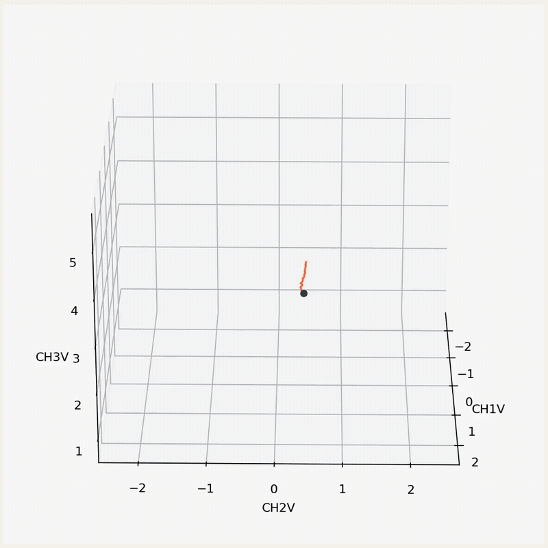
I captured the three state voltages on my Rigol DHO804 via its rear USB port using pyvisa to pull the raw waveform data, then plotted them directly as a rotating 3D reconstruction of the attractor. Enjoy!