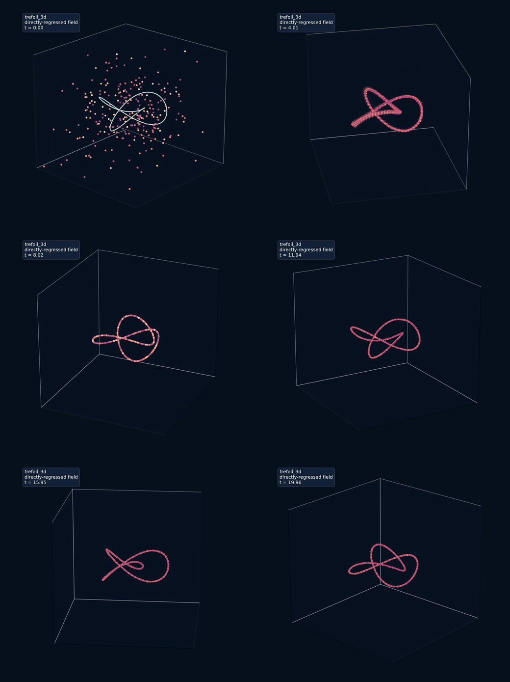
Trajectories converging onto a 3D trefoil knot
A few months back I came across an article from Unconventional AI which demonstrated how they successfully steered a simple oscillator system under a time-dependent control signal to follow a given trajectory. It got me curious about a similar question: is it possible to construct an ODE with no time dependence and no control that follows a given trajectory? In other words, is it possible to bake a desired limit cycle into an autonomous ODE? This is a different question than the one posed in the article. There, the complexity appears in the design of the control; here, it appears in the design of the system.
I got curious whether I could take the idea further. If such an ODE can be constructed, could I also realize it as an analog circuit, the way I did previously for the Lorenz system? And how would I make sure it could be built from only a few components? If we arrive at a limit cycle that is stable, this fights the unavoidable noise problems in analog computing circuits. These circuit questions are a teaser and I’ll leave the circuit build as a potential follow-up.
This post is a record of my attempt at the first goal: constructing an ODE with a given limit cycle. For simplicity I will consider a smooth, periodic parametrized curve with no self-intersections.
Recently, I’ve had fun learning the theory behind flow matching and diffusion models from this online MIT course, and it felt like the right framework for this problem. The gist of flow matching is to decide how you want a probability distribution to transform over time, and then determine the flow field that accomplishes it. What I do here is nearly identical to that standard construction, adapted to the problem at hand.
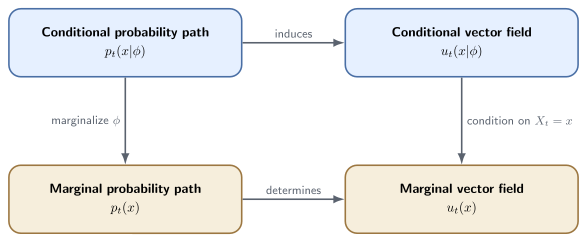
The construction is four moves, following the standard flow-matching process, and it helps to see them laid out before diving into each one. First, a conditional probability path: for a single fixed phase , a density that starts as pure noise and collapses onto one moving point traveling along the curve. Second, the conditional vector field that induces that path, which turns out to have a clean closed form. Third, the marginal probability path: average the conditional path over all phases, so the mass wraps the whole curve instead of chasing a single point. Fourth, the marginal vector field that transports it, recovered by conditioning on where a particle currently sits. That last field is the time-dependent flow I am after, and the four sections below walk these boxes in order.
This gets me close to what I want, except that the field it produces is still time dependent:
The we find drives trajectories onto the chosen curve.
I noticed in simulations that the flow appears to become steady at large times (I later show why). We then explore the idea of applying this limiting field for all time. This gets us to an autonomous ODE of the form
where approaches a desired parametrized curve and then keeps circulating along it forever, which is exactly what I was after.
If you know of other methods for finding such an ODE, I would love to hear about them, and I’ll edit this post to add a reference. From the limited literature search I did, I didn’t see anything that took the approach shown here, but it’s possible I could have missed it. Regardless, I enjoyed the challenge of trying to solve it myself.
The Conditional Probability Path
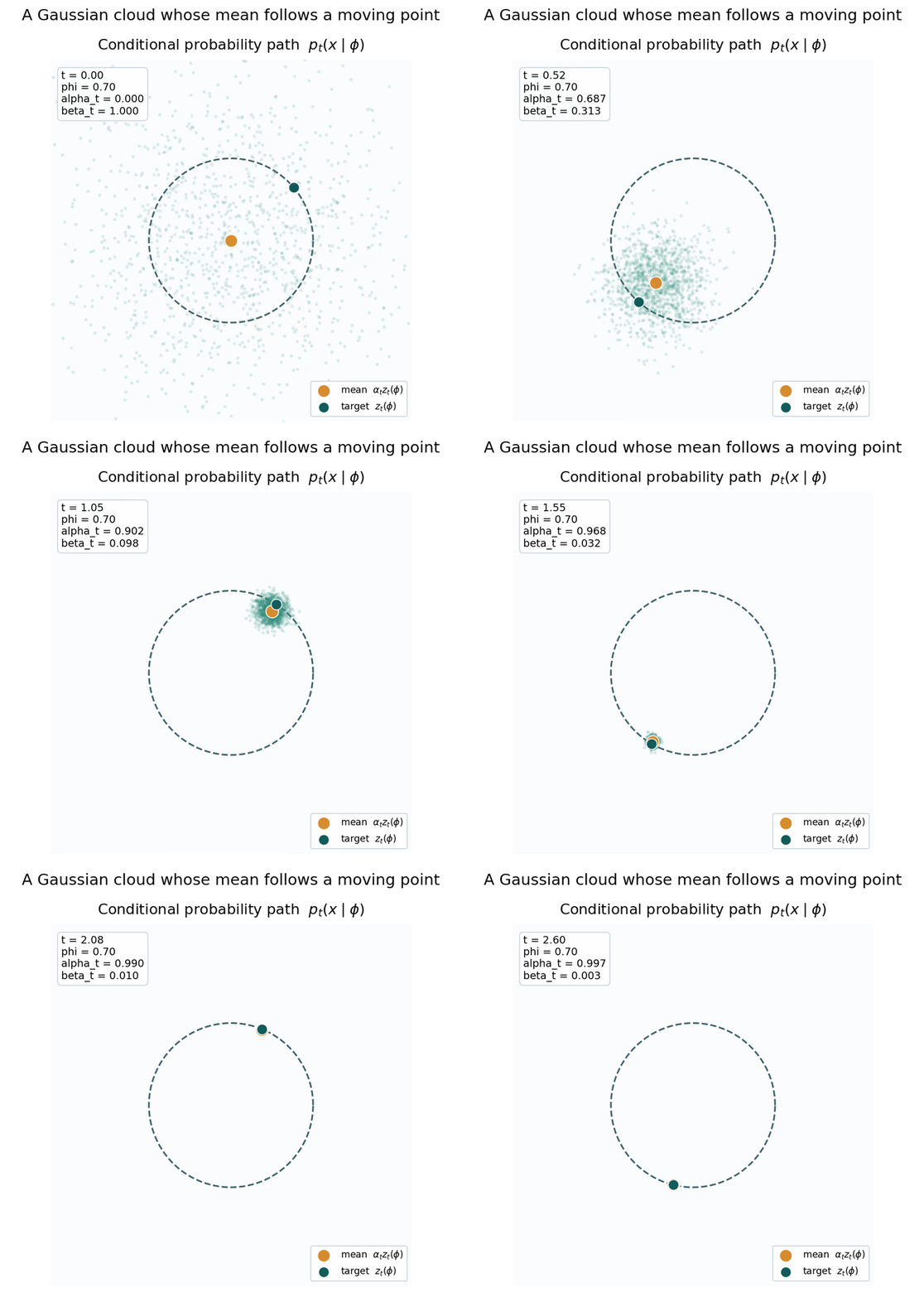
We start with the conditional probability path, which is a designed time-dependent probability density conditioned on a particular phase offset . In other words, we design a density that converges onto one moving point specified by . Covering the whole curve comes later; for now the target is a single point.
The phase picks out where that point starts, and it then travels around the curve at rate :
The conditional probability path is a Gaussian centered on that moving point, with a variance that shrinks over time:
with schedules
At early times is close to one and is close to zero, so the density is essentially pure noise. As time goes on decays and approaches one, so the density tightens around . That is the transformation we asked for: noise at the start, a point on the curve at the end.
The Conditional Vector Field
We designed the density; now we solve for the velocity field that produces it. That is the second half of the flow-matching recipe, and because the conditional path is built from an explicit formula, we can read the field straight off it.
The conditional flow map takes a starting point drawn from the noise and returns where that particle sits at time :
Differentiating in time gives its velocity:
We want that velocity as a function of where the particle currently is rather than where it started, so we substitute and use :
This has exactly two pieces, each doing something clear:
- normal term : pulls the particle toward the moving target
- tangential term : pushes it along the curve
In other words, the field pulls inward and transports along. I found this satisfying, because the algebra didn’t just hand back some velocity field, it handed back exactly the structure you’d want to design by hand. It’s worth keeping this two-piece shape in mind, because it survives every step that follows, all the way to the final autonomous field.
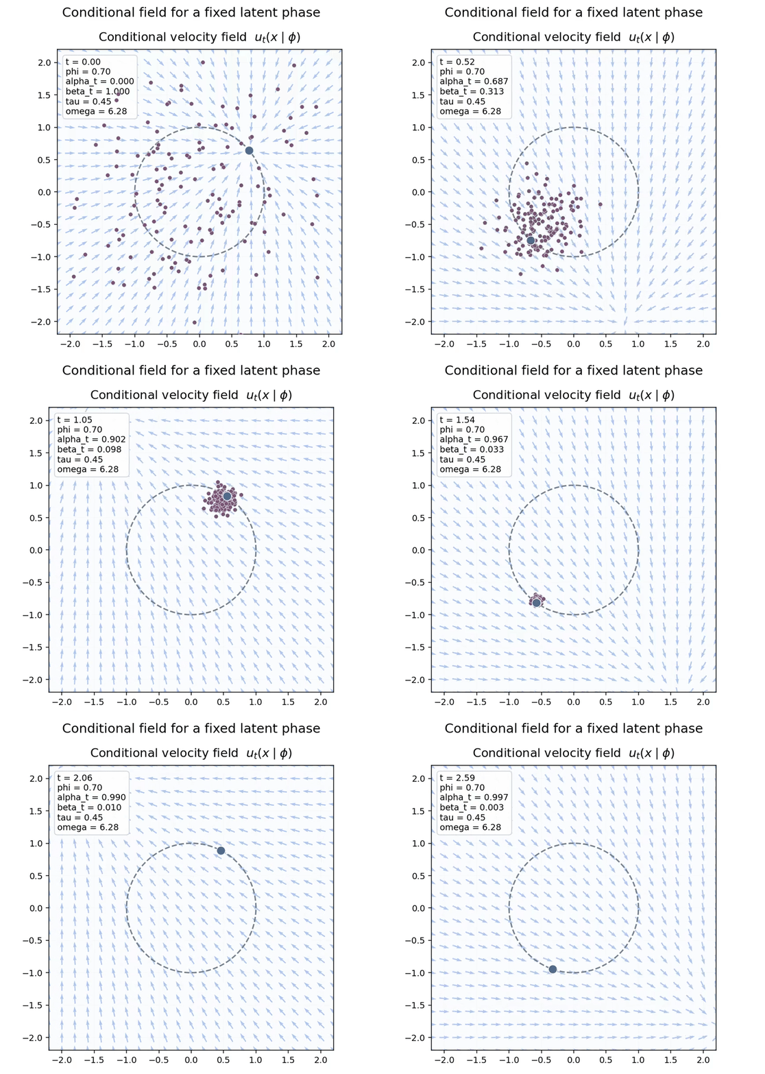
Trajectories under the conditional field for one fixed phase , together with the moving target point .
The Marginal Probability Path
The conditional path does what we asked, but only for one fixed phase : it converges onto a single moving point, not the whole curve. The fix is to stop treating as fixed and make it a random variable instead:
and marginalize the conditional path over it:
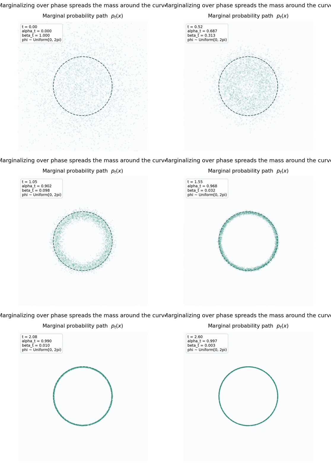
In other words, we average the conditional densities over every phase offset. Instead of one cloud chasing one point, the mass is now spread all the way around the curve. Early on the density is diffuse; as time increases, it contracts into a narrow band wrapped around the entire target. This is the probability path we actually want.
The Marginal Vector Field
Same pattern as before: we have the density we want, so now we solve for the field that transports it. The answer is not a plain average of the conditional fields, but a posterior average, weighted by which phases could plausibly have produced the point we’re standing at:
Written as an integral:
In other words: given that a particle sits at , average the velocities of all the phases that could have put it there, weighted by how likely each one is. If is near some part of the curve, the conditional fields for nearby phases dominate the average.
This isn’t a heuristic. The marginal field is exactly the field that transports the marginal density. This is shown by demonstrating that the following continuity equation holds:
At this stage, we actually don’t need to compute this integral explicitly. We can move straight to fitting a neural network to this field.
Simulating the Time-Dependent Flow
To test it I picked a nonplanar “crown” loop in , a circle with three vertical waves, and trained a small network on it:
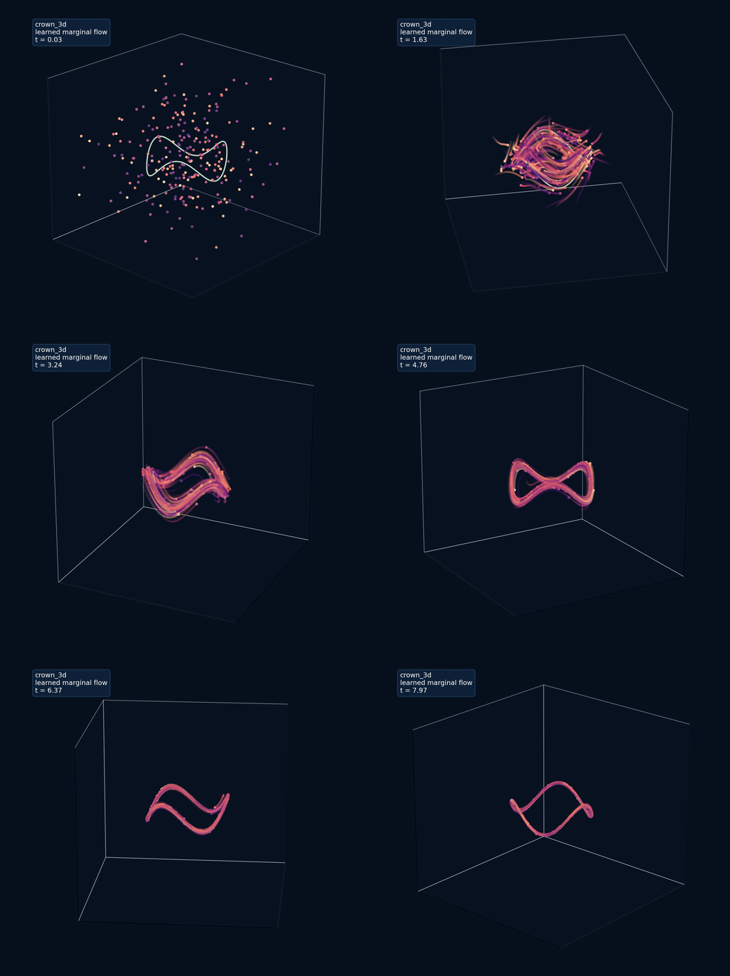
Trajectories from noise under the learned time-dependent marginal field , rendered out to .
Training follows the standard conditional flow matching recipe, and it’s short enough to describe completely. Each step:
- Sample a batch of phases , times , and noise .
- Construct the point , a sample from the conditional path.
- Regress: minimize , where the target is the conditional field derived above (which we have in closed form). See the MIT lecture notes for an explanation of why we can regress against the conditional field rather than the marginal field.
Notice that there is no ODE solving during training and no simulation in the loop. The network never sees , which is exactly why it converges to the marginal field rather than to any one conditional field. The network itself is deliberately tiny: an MLP taking with a few narrow hidden layers (SiLU activations). I used and .
To make the animation, I then draw 256 particles from and integrate with a fixed-step RK4 integrator (), rendering the cloud as it evolves.
The Marginal Flow Approaches a Steady Flow
At this point we have a flow that drives trajectories onto the curve, but one that still depends on time. Watching the simulation, though, something curious happens. After the initial collapse onto the curve, the field seems to stop changing and the cloud just circulates. That suggests the time-dependent marginal flow is settling into a steady flow (time-independent vector field), and it turns out we can show exactly that.
Time enters the marginal field in two distinct ways: through the rotating target , and through the schedules . The two disappear by completely different mechanisms: the first exactly, by symmetry, and the second asymptotically, by concentration. We take them in turn.
Step 1: the rotation dies exactly, by symmetry. Substitute
Since is uniform on the circle and the uniform measure is rotation-invariant, is also uniform, for every . The same integral rewritten over has
and has vanished. The only remaining time dependence is through and .
In other words, at any instant the ensemble of “which point is being chased” looks statistically identical. The rotation was only ever visible conditionally, and averaging over a uniform phase erases it. (This step leans entirely on the phase prior being uniform. Any other prior would leave a rotating lump in the weights, and the argument would fail.)
Step 2: reorganize as a posterior expectation. Define the Bayes weights
so that
Step 3: the schedule dies asymptotically, by concentration. As this is a Gibbs distribution at vanishing temperature: the weight piles exponentially onto whichever minimizes , and since , those minimizers converge to the nearest points on the curve.
Step 4: at regular points, the posterior collapses. If has a unique nearest point :
This is the same two-piece structure as the conditional field, but now aimed at the nearest point on the curve rather than at a latent moving target. There’s no phase left to condition on, and no schedule left to run. On the curve itself the normal term vanishes and , so the curve is an orbit of the limiting field.
Steps 1 and 2 are exact algebra, but Steps 3 and 4 are a concentration argument at physics-level rigor: I believe the conclusion at regular points, but it breaks down exactly where you’d expect, at points equidistant from multiple parts of the curve, where the posterior refuses to pick a single branch and the limit is a blend of competing velocities.
Using the Limit for All Time
We derived as a limit, but nothing stops us from simply using it as the field for all time, starting from noise at :
This is the autonomous ODE I set out to construct. The follow-the-curve guarantee from earlier belonged to the time-dependent flow; the continuity equation says nothing about running the limiting field from . So what follows is an experiment, but one piece of theory backs it up.
Orbital Stability: A Stable Limit Cycle in the Tube
Here is a short argument, at the same physics level as the rest of this post, that the curve is a stable limit cycle of . Track half the squared distance to the curve along a trajectory:
Stay in a thin tube around the curve, close enough that the nearest point is unique. Two geometric facts do all the work there. The gradient of is the vector from the nearest point back to ,
and that vector is perpendicular to the tangent — if it weren’t, sliding the foot of the segment along the curve would find a closer point. Now differentiate along a trajectory: the perpendicularity kills the tangential term, and the normal term hands back itself:
This is an exact identity, not a bound: inside the tube, distance to the curve decays as , everywhere at the same rate. Notice how the two-piece structure splits the labor — the normal term does all the stabilizing, while the tangential term only sets the speed of traffic around the loop. And since the normal term vanishes on the curve itself, the curve is a periodic orbit. A periodic orbit whose neighborhood drains onto it exponentially is a stable limit cycle.
The argument is local by construction: it lives in the tube where the nearest point is unique, and says nothing at points tied between two parts of the curve, where is discontinuous. Starting from noise, far away, do trajectories converge? That global question is not proven (maybe the reader can try!). I’m content for now just trying it out in simulation.
Simulating the Autonomous Field
The deliverable is an autonomous ODE I can actually run: a compact, differentiable network approximating , with no time input and no lookup table to carry around.
For the time-dependent field above I used the standard flow-matching move, regressing against the conditional field and letting the hidden phase average into the marginal. That trick earns its keep when the target is a field you cannot write down. Here we can: is closed form, needing only the nearest point on the known curve. So there is nothing to gain from the conditional trick, and worse, it would hand back a smoothed version of rather than the sharp field. Instead I regress on directly: sample points at a range of distances from the curve, evaluate the exact at each by nearest-point lookup, and fit to it.
In practice, I didn’t have an issue with discontinuities or points equidistant from the curve. If a given curve presented this issue, we could regress against a smoothed version which would be equivalent to the marginal time-dependent field fixed at some large finite time .
The gain is that this decouples where I sample from what I fit. Sampling only has to cover where trajectories go, from right on the curve out to where noise starts, while the target is the sharp everywhere, so nothing gets smoothed. A small MLP, on the order of parameters, trained this way gives an autonomous field with no time input anywhere. The only gap left is the network’s own fitting error, with no formal guarantee that the learned field keeps the curve as a stable limit cycle, only the objective’s promise that . To draw a simulation I integrate from pure noise with a fixed-step RK4 solver.
Gallery
The learned autonomous field integrated from pure noise, on six target curves. Each is its own network, trained by the recipe above; the only thing that changes is .
The Crown
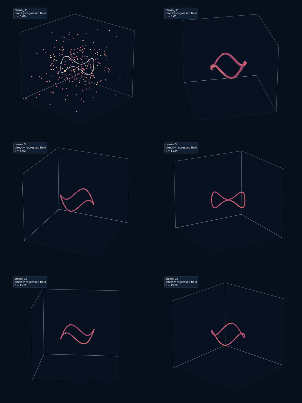
Trajectories from noise onto the crown, out to .
The Trefoil Knot
Trajectories from noise onto the trefoil knot, out to .
The Loop
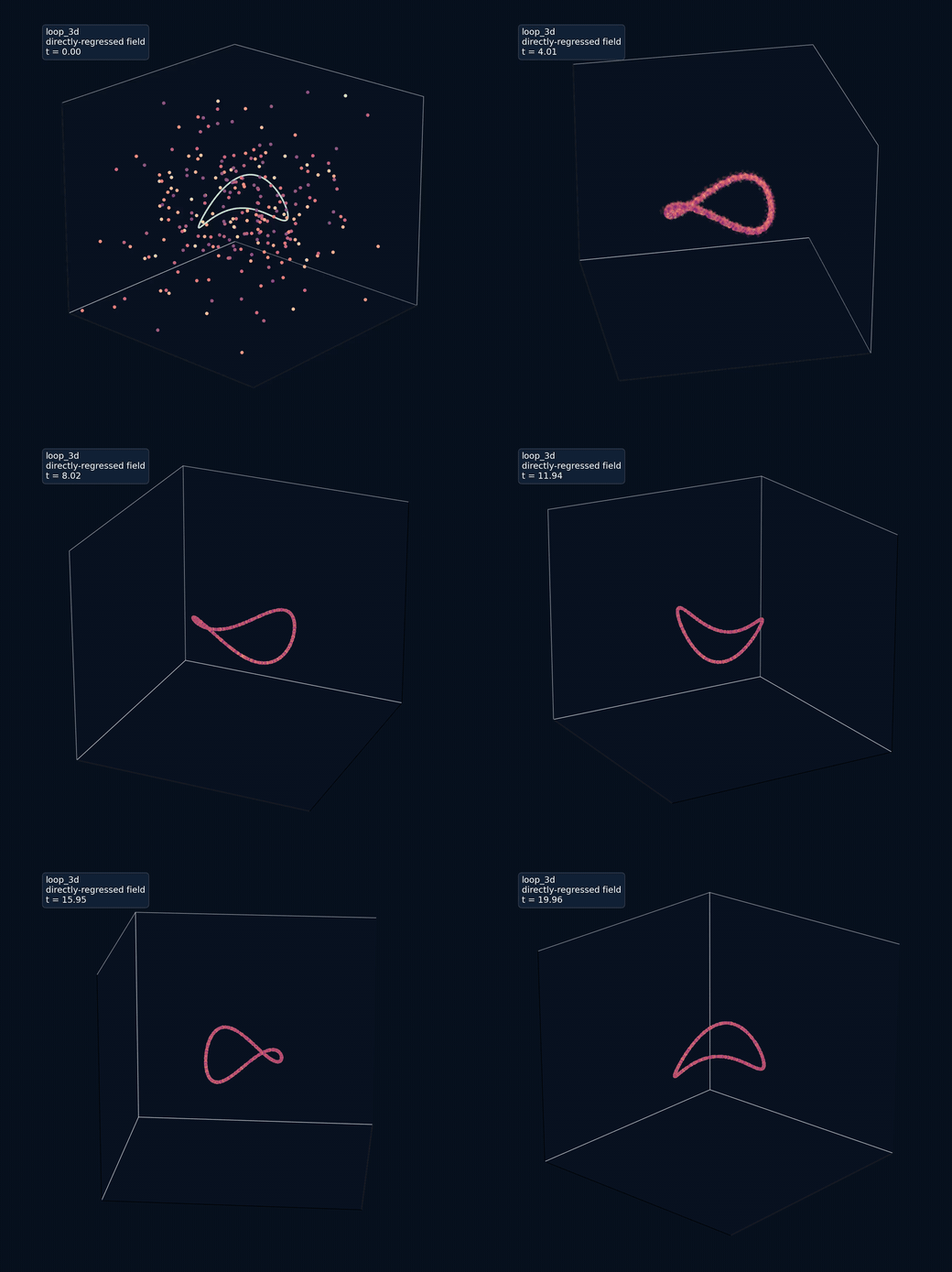
Trajectories from noise onto the loop, out to .
The Rose
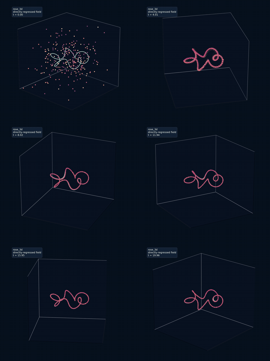
Trajectories from noise onto the rose, out to .
The Figure-Eight Knot
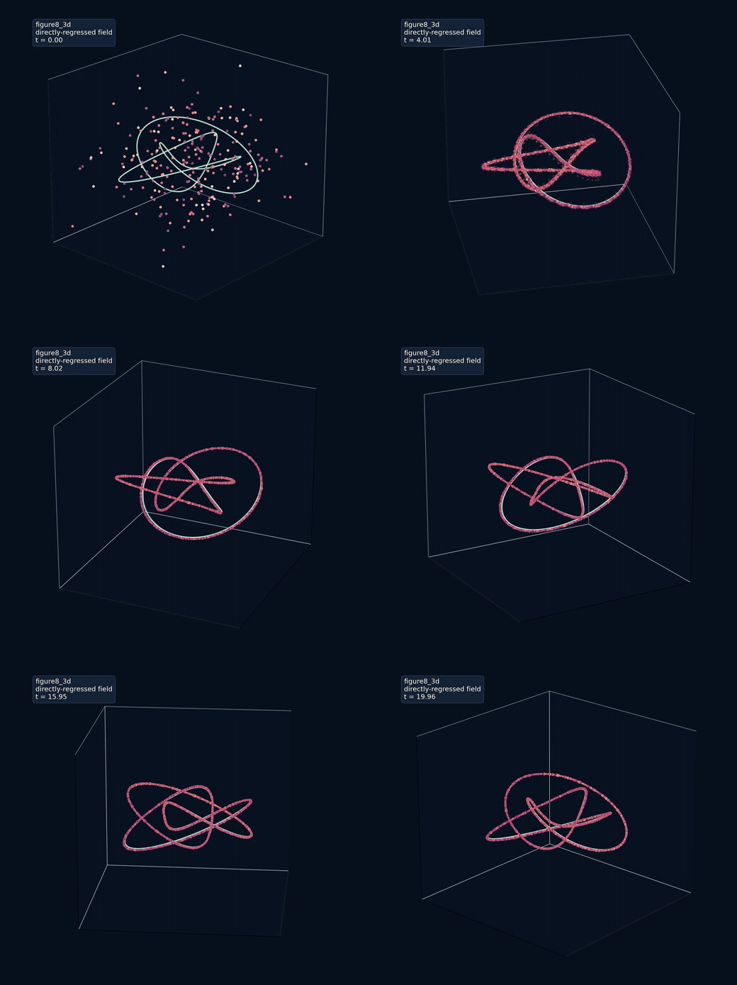
Trajectories from noise onto the figure-eight knot, out to .
The Baseball Seam
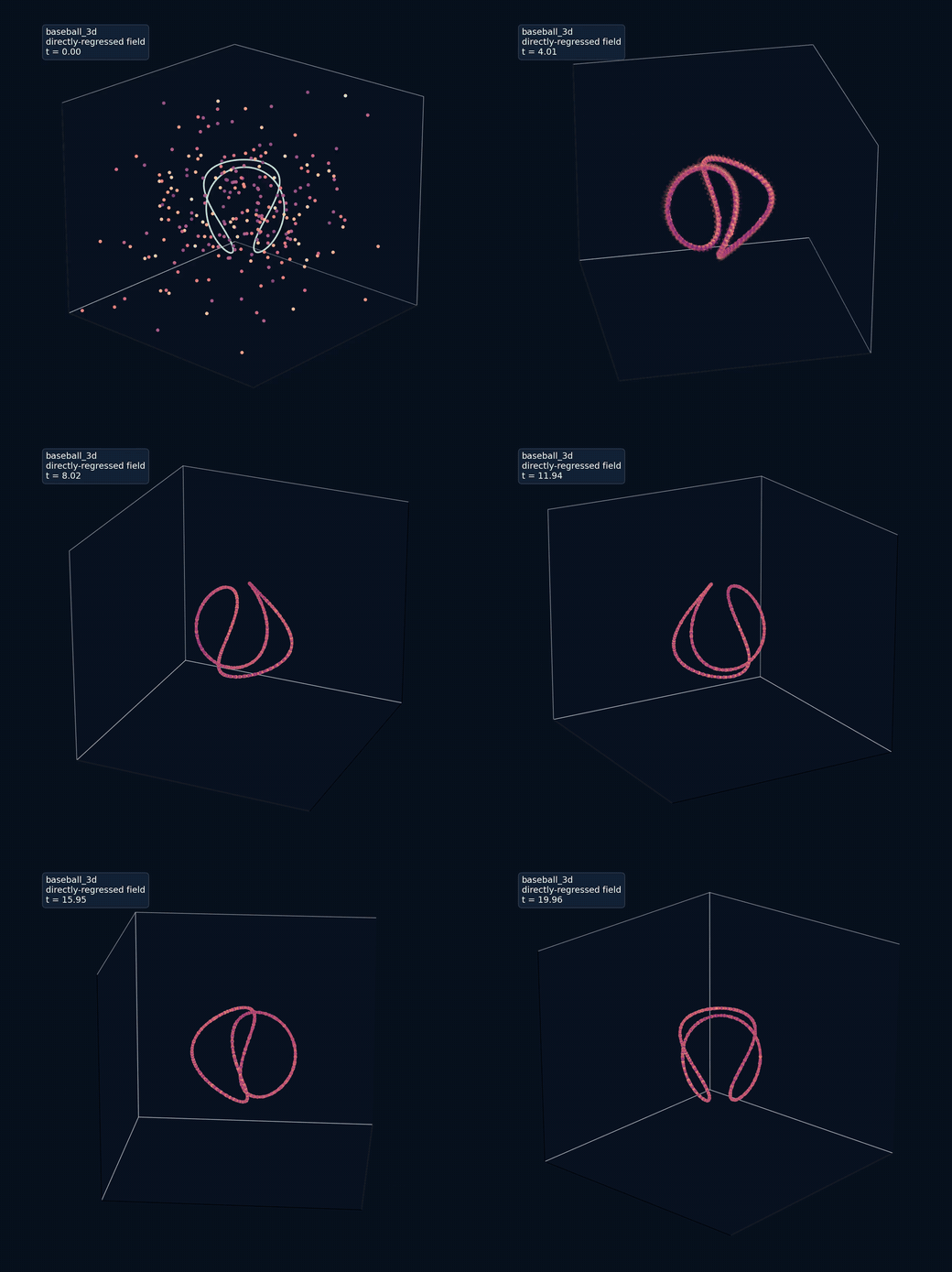
Trajectories from noise onto the baseball seam, out to .
What’s next?
Next, I want to see if I can distill as a low-order ODE that is buildable with a few analog components like in the Lorenz circuit. The SINDy algorithm (sparse identification of nonlinear dynamics) looks like the right tool, and that’s where I want to take this next. With a low-order distilled ODE, this could also give us hope to show global stability beyond the local arguments here.