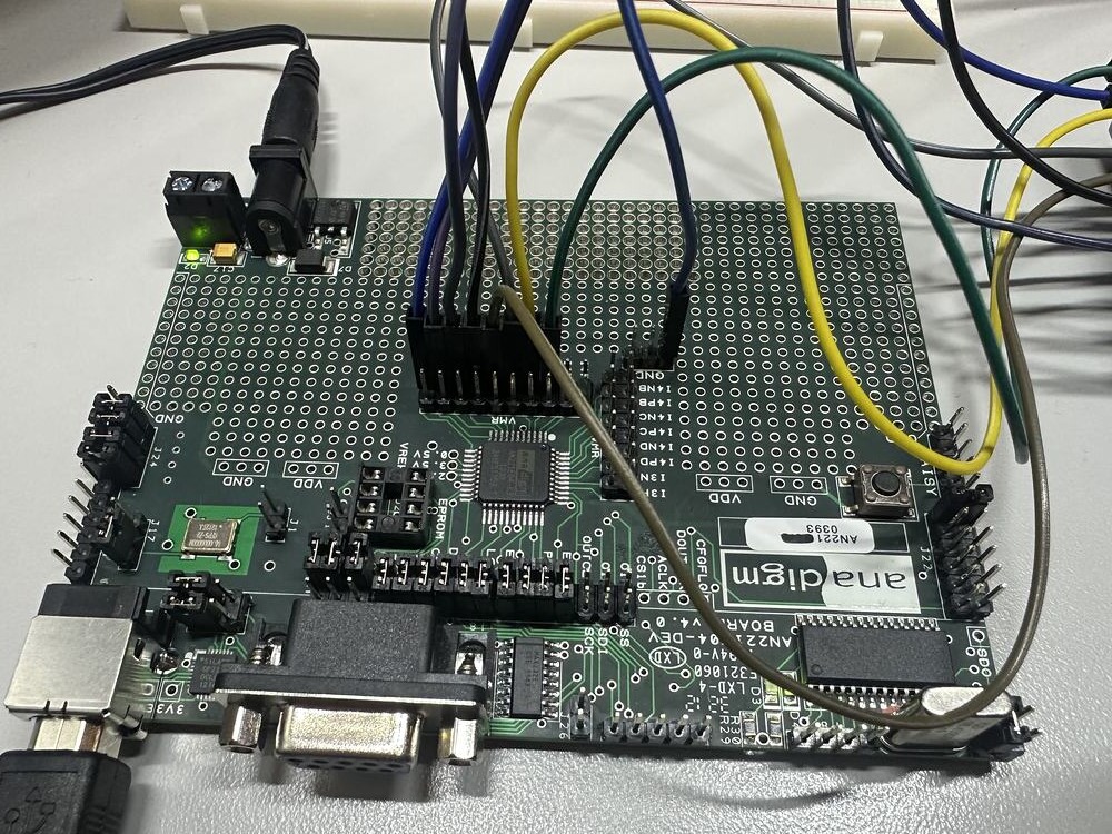
Here I dive into the world of thermodynamic computing realized on a field programmable analog array, or FPAA for short.

First, I want to introduce these possibly foreign concepts to the reader who may have stumbled upon this page. What is an FPAA exactly? What is thermodynamic computing?

An FPAA is the analog version of its cousin the FPGA, the field programmable gate array, which is aimed at digital design. An FPAA allows for prototyping analog circuits in software and reconfiguring an analog circuit design over USB. This allows for quick prototyping of various designs without having to physically wire each design on a breadboard or perfboard by hand. I’m using an AN221E04 (quite an old board released in 2004) which internally has analog components (such as amplifiers, capacitors, summers, integrators, and so on) that can be wired and parameterized in software. It has configurable analog blocks (CABs) connected through a programmable routing network. Many functions are implemented using switched-capacitor techniques. A switched-capacitor circuit uses a capacitor and periodically controlled switches to move charge in discrete steps, which makes it behave like a programmable resistor or other analog element.

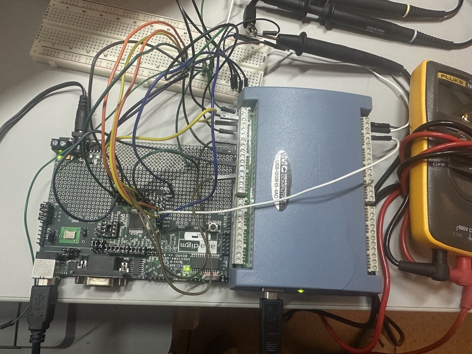
What is thermodynamic computing? It is a form of computing that uses noise as a computational resource. This processing unit is based on the design of Normal Computing’s SPU (their first prototype before their more recent processor CN101). My goal here is to implement the same SDEs and ODEs. However, the mapping to hardware is very different between the SPU and the FPAA. The SPU constructs the ODE physically through a network of capacitors and resistors, while the FPAA uses switched-capacitor components to mimic op-amp circuit design. The SPU handles both underdamped and overdamped cases of the Langevin dynamics, while the build here implements the overdamped case only. The FPAA doesn’t have a native noise source on chip, so I create a pseudorandom Gaussian noise source that is streamed via a DAQ (data acquisition) device. This DAQ can both output analog signals and receive inputs from the FPAA chip so I can analyze the results.

The goal of this project is to build out my own thermodynamic processing unit on an FPAA so that I can have a test bed for exploring this field further. I tend to learn better by building. In this project, I implement the following linear algebra algorithms from Normal Computing’s work here:

• $A^{-1}$ algorithm
• $Ax = b$ solver

Inspired by the $Ax = b$ solver, I also consider a class of problems that operate under the same principles and give a dynamical systems stability perspective on how they work. These algorithms include:

• Finding the roots of a quadratic polynomial: $ax^2 + bx + c = 0$
• $\sqrt{x}$
• Reciprocal $1/x$

Lastly, I explore the idea of composing functions and show how you can construct $1/\sqrt{x}$ from the above primitives.

Build

Reconfiguring the chip from a script

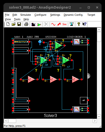
The design tool for the FPAA, AnadigmDesigner2, is a GUI you’d normally click through: drag blocks onto a schematic, set parameters in dialog boxes, hit a button to send it to the board. It also exposes a COM automation interface, and the language it expects is VBScript. So instead of clicking, I have Python write the VBScript.

A small model of the circuit works out where each block goes, what its parameters are and what connects to what, and emits a script that adds the chip, places the blocks, wires their contacts, sets the clocks and tells the chip to download. Running that script sends the design to the board with me out of the loop.

Placement and wiring only need to happen once. After that the script loops over however many systems it was handed, changing parameters and downloading a fresh bitstream each time, so the tool starts once rather than once per point. That’s what makes a sweep of a few hundred configurations possible.

The conversion from an SDE form to a circuit of integrators, summers, and multipliers is very similar to the method I used in my previous post on solving the Lorenz equations with an analog circuit.

Setting up the noise

The chip has no noise source of its own, so the DAQ makes it. Three of its analog outputs stream independent seeded Gaussian sequences, one into each state.

What the chip receives isn’t quite white noise though. The DAC picks a new value every 10 µs and holds it flat in between, so it’s really a staircase. The step height, 150 mV here, and the step width together set the effective temperature, a single noise strength $D$ that the results below depend on.

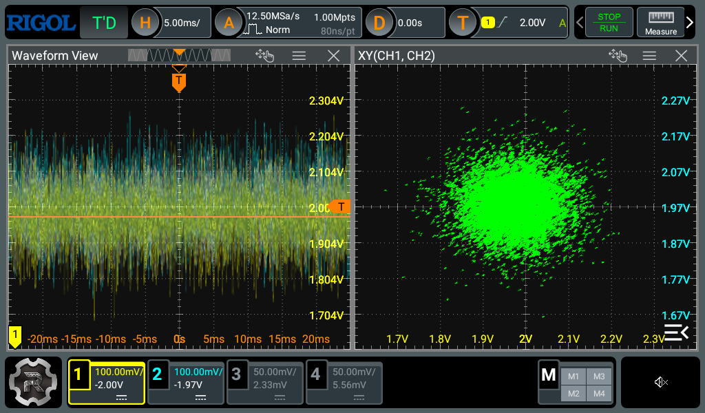
Reading the answer back out goes through the same DAQ. Each state leaves the chip as a differential pair of pins sitting either side of a mid-rail reference, so the state is the difference between them, and the DAQ digitizes both.

Key differences between FPAA and SPU

Here are some key differences between the FPAA and SPU designs.

	SPU	FPAA
unit cell	LC resonator, noise current source	summing stage + integrator
dynamics	second order, underdamped	first order, the overdamped equation directly
matrix realized as	capacitor bank	switched-capacitor design
noise	FPGA	DAQ
readout	onboard ADC, 12 MHz	external DAQ, 50 kS/s
size	8 cells	3 states

Results

Computing $A^{-1}$

The inverse and the solve come from the same circuit, and in fact from the same run. One summing stage and one integrator per row of the matrix build

$dz = (-Az + b)\,dt + \sqrt{2D}\;dW,$

where $W$ is a Wiener process and $D$ is the diffusion coefficient. For symmetric positive definite $A$ this settles into a stationary distribution

$z \sim \mathcal{N}\!\left(A^{-1}b,\; DA^{-1}\right),$

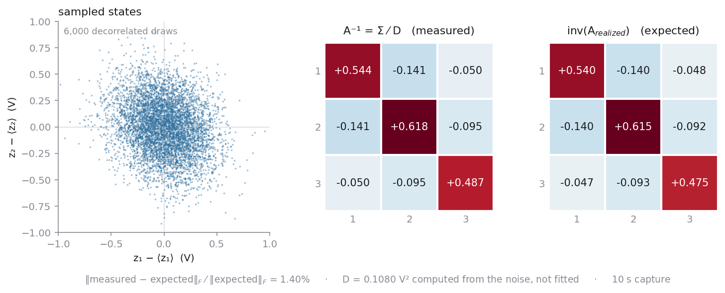
and both of its moments are answers. The mean is the solution to $Ax = b$. The covariance, divided by $D$, is the inverse. So one capture of the fluctuating state gives both: the average of the samples and their spread.

Ten seconds of samples gave the inverse to 1.4%. Measuring it the obvious way instead, one column at a time by solving with $b$ set to each unit vector, needs three separate builds and landed at 3.4%.

If the solve is all you’re after, you can turn the noise source off. Some noise is always left even then, but what remains follows $\dot z = -Az + b$ closely enough that the circuit settles at $A^{-1}b$ and stays there, so the answer is read directly instead of averaged out of a cloud. That’s how I ran the sweep: over 24 random symmetric positive definite systems the median error was 6.4% and the worst 19.6%, uncorrected.

Solving $Ax = b$ is the same thing as minimizing the quadratic $\tfrac12 x^{\top}\!Ax - b^{\top}x$, whose gradient is exactly $Ax - b$. So the circuit is rolling downhill on that surface, and its trajectories are gradient flow. To watch it I slowed a two state solver to about a millisecond and kicked it out to twelve starting points, using the noise inputs as a step generator rather than a noise source, then released it.

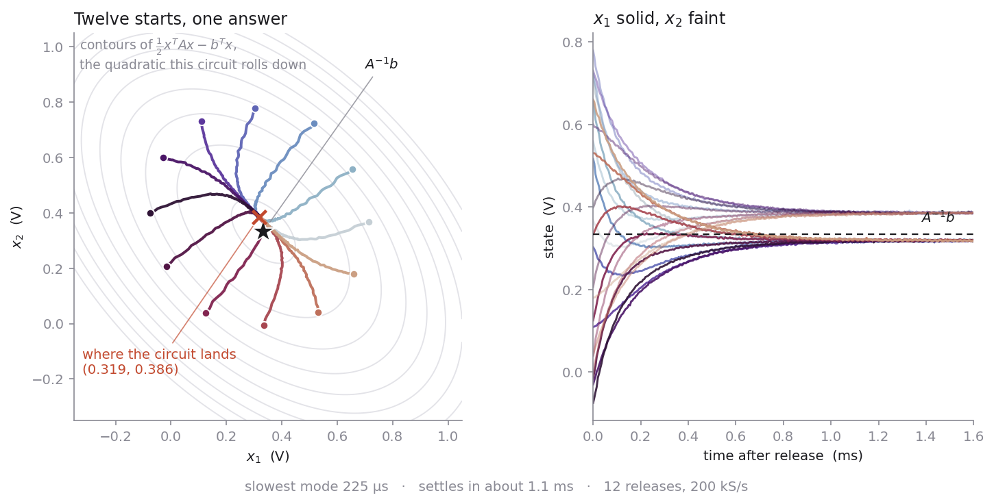
The trajectories are worth more than the endpoint. Fitting $\dot x = -Ax$ to them recovers the matrix itself, not just $A^{-1}b$, and it comes back symmetric and within 2.6% of what I asked for, with every entry low by about the same few percent as the gains elsewhere in this post.

The two moments of that one capture are worth comparing. Its mean is off by more than a third on the middle state, while the covariance built from those very same samples is right to 1.4%. A covariance is measured about the sample mean, so a constant offset subtracts out of it exactly, and the error that dominates the first moment doesn’t appear in the second at all.

Algorithms based on stable fixed points of an ODE

The $Ax = b$ result doesn’t really depend on the equation being linear. Any $\dot x = f(x)$ ends up at a root of $f$, provided that root is stable, meaning $f'(x^*) < 0$ so small displacements decay, and provided you start inside its basin. So if you can build a circuit whose $f$ has your answer as a root, the circuit computes it by relaxing. Here are three.

Roots of a quadratic polynomial

$\dot x = s\,(ax^2 + bx + c), \qquad s = \pm 1.$

The fixed points are the two roots. Differentiating at a root gives $s\,a\,(x_\pm - x_\mp)$, which has opposite signs at the two roots, so exactly one of them is stable and which one depends on the sign of $s$. Flipping the sign of the whole right hand side moves the circuit to the other root, and both roots come out of one design.

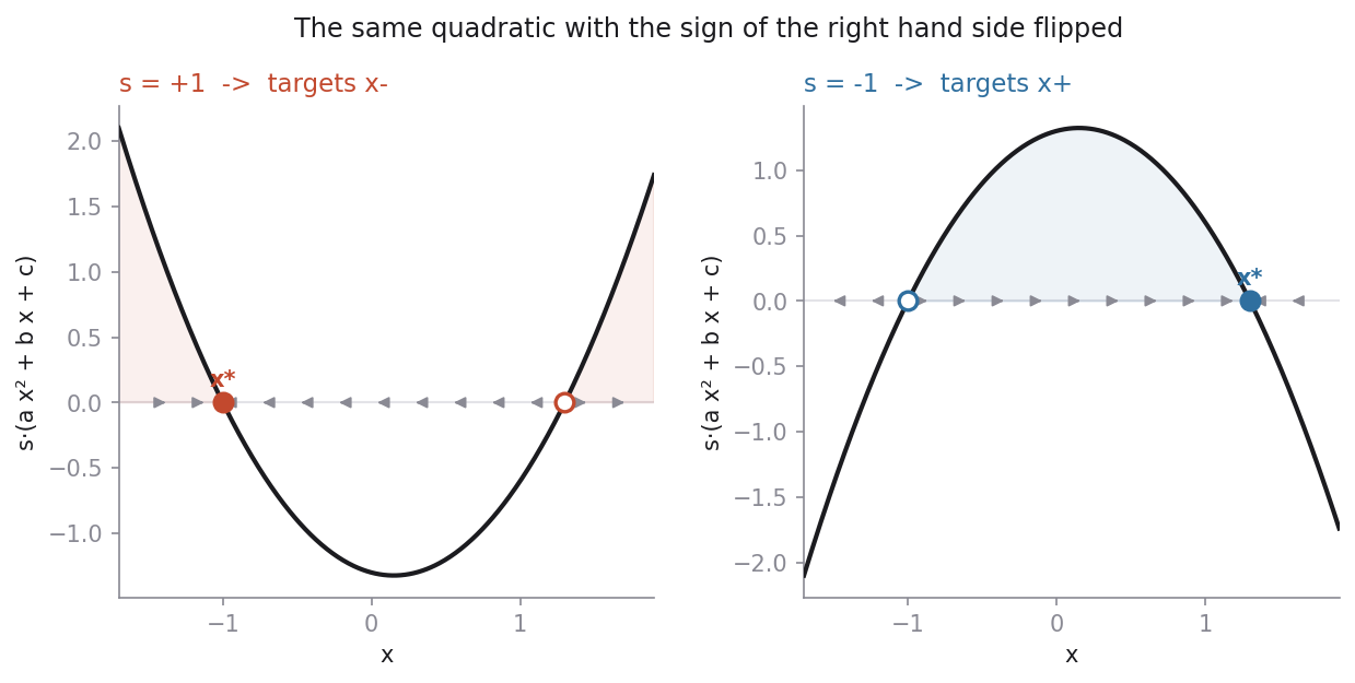
The integrator starts at zero, so the roots have to straddle zero for the circuit to reach them from there. Over ten root pairs at each sign, the largest error in the twenty measurements was 41 mV.

Square root

$\dot z = a - z^2 \;\longrightarrow\; z^* = \sqrt{a}.$

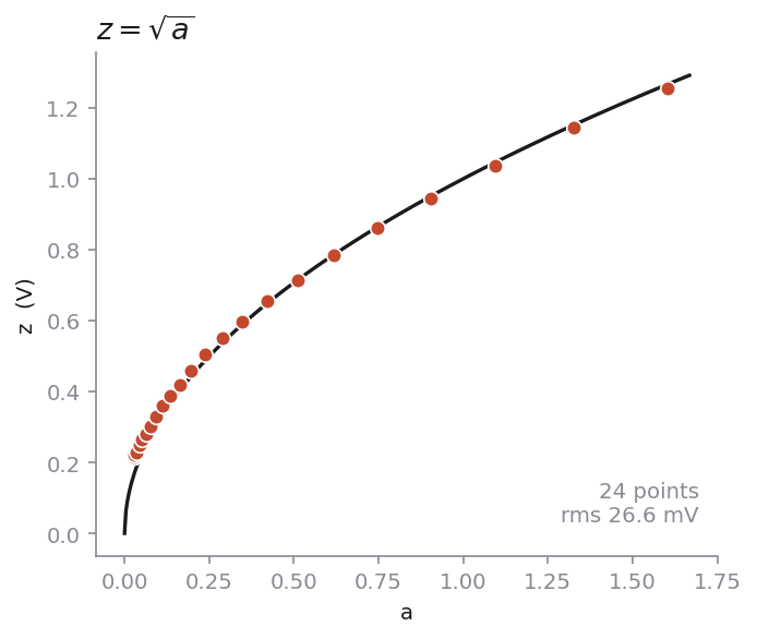
Two fixed points, at plus and minus the root, and only the positive one is stable, so a circuit started from zero can only land there. One multiplier squares the state and a summing stage subtracts it from the input.

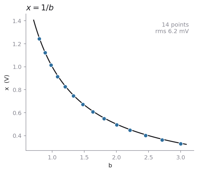
Reciprocal

$\dot x = 1 - bx \;\longrightarrow\; x^* = 1/b.$

The linear solver with a single state, and the cheapest circuit here: no multiplier at all, since the only product it needs is the state times a fixed gain.

Composition

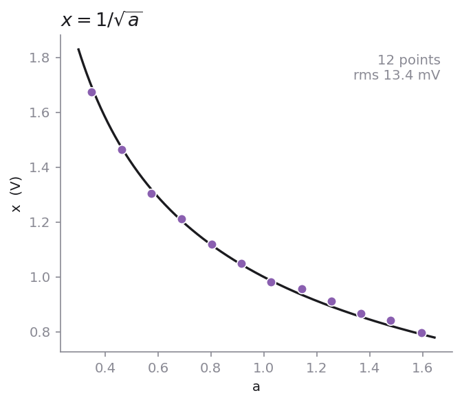
Wire the output of one of these circuits into the other and you don’t get two circuits, you get one coupled system:

$\begin{aligned} \dot z &= a - z^2, \\ \dot x &= c - z\,x, \end{aligned}$

whose fixed point is $z^* = \sqrt{a}$ and $x^* = c/\sqrt{a}$. The two stages evolve simultaneously, not one after the other.

Conclusion

Here we demonstrated that it’s possible to build a thermodynamic computer from an FPAA and a DAQ. Now that I have actual hardware capable of thermodynamic computing, it’s time to play with some noise.